

I wanted to change up what we have been looking at recently and move towards some of the potentially more useful and beneficial analyses we can perform within R. Particularly how we can look to analyse raw GPS data to create our own metrics outside of the manufacturers software. This allows us to look in more depth at the data whole also putting us in the position of not being reliant on the manufacturer to have the metric present for us to investigate it.
In this example I will go through how we can take GPS data measured at 10 hertz and manipulate it to give us a minute by minute breakdown of the data. As shown here these demands can very greatly between sport and by position within a sport. Having a better understanding of these demands puts us in a more informed position for both training and rehabilitation. For the example I have put together a set of GPS data with only a time and speed column, as what data is available in raw form can vary with manufacturer I have tried to demonstrate using the basic data every export should have.
The steps involved will be:
- Read in file.
- Create threshold based speed data (optional).
- Create column for time between data points.
- In theory you could use 0.1 seconds (10 hertz data implying 1 data reading per 0.1 seconds) for this however I have found some GPS brands vary considerably here with some having more consistent time between data points than others.
- Create column for distance covered between data points.
- Create column to split data into minutes.
- Create data frame with distance covered each minute.
The packages required are as follows:
- library(tidyverse)
- library(zoo)
- library(magrittr)
- library(lubridate)
- library(stringr)
And the code:
- ###Read csv
- raw_gps <- read.csv(file=file.choose())
- ###Add Speed Threshold if desired
- raw_gps %<>% mutate(“SpeedHS” = case_when(Speed.m.s <= 5.5 ~ 0, Speed.m.s > 5.5 ~ Speed.m.s))
- Using the ‘case_when’ function is similar to an ‘if’ formula in Excel. Here we create a second speed column which changes values less than 5.5m/s to zero and keeps values above it the same.
- raw_gps %<>% mutate(“SpeedHS” = case_when(Speed.m.s <= 5.5 ~ 0, Speed.m.s > 5.5 ~ Speed.m.s))
- ###Time between datapoints
- raw_gps$Time <- strptime(raw_gps$Time, ‘%H:%M:%OS’)
- Important to have milliseconds in time, denoted by %OS instead of %S
- raw_gps$Time_diff<-c(0, diff(raw_gps$Time))
- raw_gps$Time <- strptime(raw_gps$Time, ‘%H:%M:%OS’)
- ###Distance at each datapoint
- raw_gps$dist <- raw_gps$Speed.m.s*raw_gps$Time_diff
- raw_gps$hs_dist <- raw_gps$SpeedHS*raw_gps$Time_diff
- Speed*time=Distance.
- ###Time chunks
- raw_gps$one_Min <- cut(raw_gps$Time_elapsed, breaks = seq(-1, max(raw_gps$Time_elapsed), by = 60))
- One minute chunks using the ‘cut’ function
- raw_gps$two_min <- cut(raw_gps$Time_elapsed, breaks = seq(-1, max(raw_gps$Time_elapsed), by = 120))
- Two minute chunks
- raw_gps$Time <- NULL
- Time column may cause issues at next step so remove if necessary
- raw_gps$one_Min <- cut(raw_gps$Time_elapsed, breaks = seq(-1, max(raw_gps$Time_elapsed), by = 60))
- ###Dist Per Min/Dist Per 2 Min
- Min_by_min <- raw_gps %>% group_by(one_Min) %>% dplyr::summarize(TotalDist_Min=sum(dist), Total_HS_Dist_Min=sum(hs_dist))
- Min_by_min2 <- raw_gps %>% group_by(two_min) %>%
dplyr::summarize(TotalDist_Min=sum(dist), Total_HS_Dist_Min=sum(hs_dist))- The above ‘summarize’ formula sums the distance covered within the different time chunks created previously.
- ###Check to ensure total distance is same for both
- sum(Min_by_min$TotalDist_Min)
- sum(Min_by_min2$TotalDist_Min)
- Quick check to validate analyse by ensuring both data frames have the same total distance covered.

Script P1 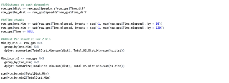
Script P2
That was a relatively short way to create usable data from raw GPS data. With this short approach we can branch out and create time periods within the data (isolate 1st/2nd half, drills within training etc.), individualise analysis for players, add more detailed metrics such as average acceleration or mechanical work or even look to incorporate tactical analysis data such as involvements, passes, tackles etc.
PS: As a bonus here is a basic ggplot code which outputs the graph shown above:
- ggplot(data=Min_by_min, aes(x=one_Min, y=TotalDist_Min, fill=TotalDist_Min))+
geom_bar(stat = ‘identity’)
Note to carry this analyse out on a number of players, separating the data into lists is the best approach.
Part 2: Analysing multiple files
Part 3: Adding Rolling Average Data
Update – 30/01/2019
The above outlines how to produce minute by minute data. I covered this approach here as R was still new to the blog and it’s a short process to outline. However, extracting peak period data through this manner is not the most accurate as it aggregates the data to minute periods. To be more precise, we must stay at the 10Hz data and producing rollin sums of the distance covered for each datapoint. This approach is outlined across 2 posts as it involves more detailed work in R along with specific steps taken to reduce the time needed to carry out the analysis. If the above approach was applied to 10Hz data, it would take over 10 minutes for 20 players data to analysed. The approach designed can work through the same amount of data in around a minute.

Very good , which gps brand are you using? Stastports, Catapult, WImupro, gpexe?
LikeLike