How To Produce Minute By Minute Data From 10Hz Data – Multiple Files

After this post last week I had a few questions on twitter about implementing the analysis with a large number of exports present. I mentioned it briefly at the end of the blog but I have found using lists the best approach here as it prevents data from one athlete affecting the data of another. Depending on your GPS system, your export format may be a single file with all players included or individual exports per player. The overall approach for both is the same however the first steps differ.

Single file:

Reading the data into r here is identical to what we looked at previously, however we will then separate the large data frame we have created into a list of data frames separated by player name.

• raw_gps <- read.csv(file=file.choose())
  • Reads raw data into r
• df_list <- split(raw_gps, list(raw_gps$Player.Name), drop=T)
  • Separates into list of dataframes by player name.
  • ‘drop=T' ensures the data is kept in data frame format and not changed to matrices

Multiple Files

This I found a bit more complicated as we need to keep the filename involved in the data here. When we have multiple files often the athletes name isn’t included in the data itself and we miss out on having a variable to differentiate between athletes.

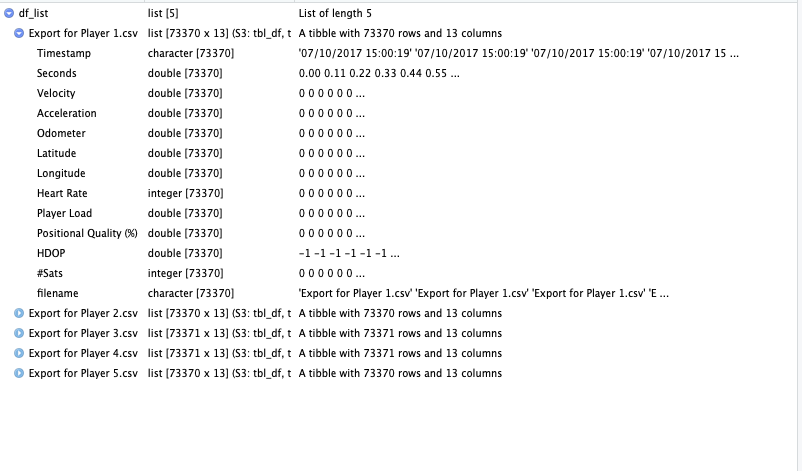
• df_full <- list.files(path="/Users/username/desktop/testfolder 2", pattern="*.csv", full.names = T) %>% map_df(function(x) read_csv(x) %>% mutate(filename=gsub(" .csv", "", basename(x))))
  • The first step is the most complicated where we first list all the file names (list.files), then create a large data frame (map_df) which combines all the files into one and create a column which is equal to the filename (mutate)
• df_list <- split(df_full, list(df_full$filename), drop=T)
  • The next step is the same as above where we split it into a list of dataframes based off the filename.

The next few steps will be very similar to how we worked through the data previously however all the script all have the lapply wrapped around them. This lets us apply a function over items within a list.

• ###Time between datapoints
  df_list2 <- lapply(df_list2, function(x) {x$Time_diff<-c(0, diff(x$Seconds));x})
• ###Distance at each datapoint
  df_list2 <- lapply(df_list2, function(x) {x$dist <- x$Velocity*x$Time_diff ;x})
• ###Time chunk
  df_list2 <- lapply(df_list2, function(x) {x$one_Min <- cut(x$Seconds, breaks = seq(-1, max(x$Seconds), by = 60));x})

The above script creates the distance covered at each datapoint and the minute blocks within the data. Within each line we are saying for every item within the list called df_list2, apply a function, which we then outline and finally ;x is telling it to return the item following the function.

The next step is slightly more complicated as previously we only needed to group by the minute blocks and sum up the distance covered within, now we need to repeat this across multiple dataframes within the list.

• ###Dist Per Min/Dist Per 2 Min
  Min_by_min <- df_list2 %>% bind_rows(.id="id") %>% group_by(id, one_Min) %>%dplyr::summarize(TotalDist_Min=sum(dist))
  • bind_rows binds all the dataframes in the list together into one data frame and creates an ‘id’ column which links the data back to the original data frame it came from. By then using this ‘id’ column within the group_by we keep each individual athletes data separate from each other.

The next step is how you want the data to be output. We can write a single csv file with all the athletes together or write multiple csv files, with each athlete have a separate output.

• write_csv(Min_by_min, path='/Users/username/desktop/testfolder 2/Output/all.csv')
  • Single csv named ‘all.csv’
• df_list_final <- split(Min_by_min, list(Min_by_min$id), drop=T)
• mapply(function (x,y) write.csv(x, file = paste0('/Users/username/desktop/testfolder 2/Output/', y, '.csv'), row.names = F), df_list_final, names(df_list_final))
  • Multiple csv files, first split data into list, then we write to csvs using mapply function, with the name of the separate dataframes also the name of the output csv.

PS – Note ‘skip=8’ included in the read_csv line as a popular GPS system includes information in the first few rows which prevent the file loading in the correct format into r.

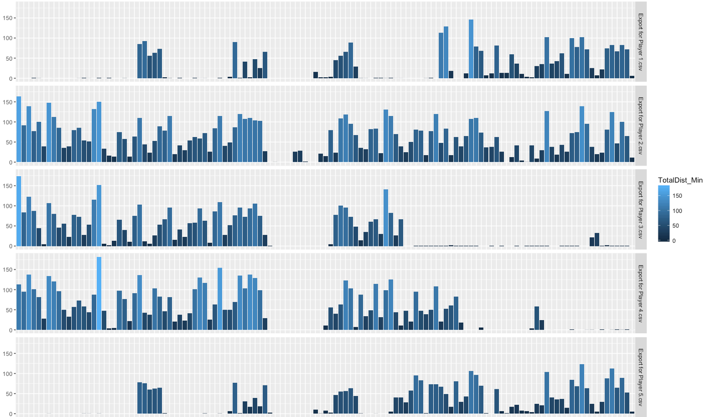
As before to generate the above plot the script is:

ggplot(data=Min_by_min, aes(x=one_Min, y=TotalDist_Min, fill=TotalDist_Min))+geom_bar(stat = 'identity')+
facet_grid(id~.)