

Much of what we have looked at previously in R has been based around GPS data, today I thought we would look at a different source of data. Various forms of monitoring is available through heart rate data, with HRV based testing being quite common, we will be looking at rMSSD data in particular here. We will also step away from the script based work in R and look at what is possible with Markdown when it comes to creating reports.
Note: To produce pdfs from RStudio you need to have a software designed for LaTeX installed. See here for Mac based MacTex instructions or here for Windows based MiKTex
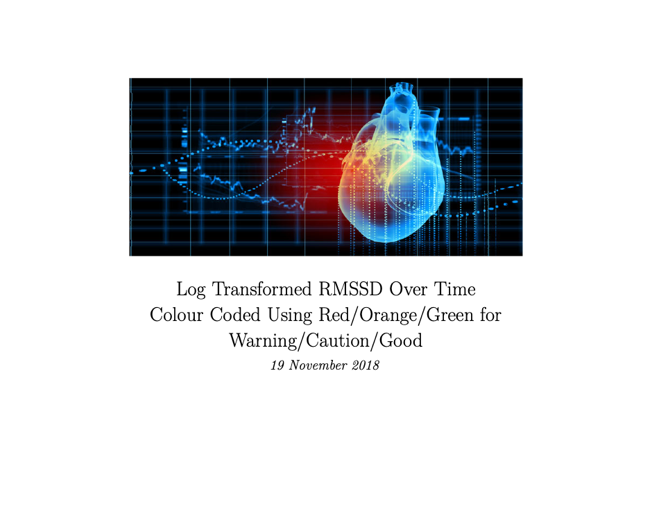
Here is a sample report produced through Markdown looking at HRV data with both a table for the most recent data from each athlete and individual graphs displaying trends plus highlighting data-points of concern.
While there is script present in the markdown script for the report we haven’t looked at previously, hopefully by working through it in a step-by-step approach you can start to see how this approach may useful in your work. In order to highlight the markdown elements of the script, some of the other areas such as the data wrangling and plotting will be simplified from the script used to create the example pdf.
Title Page
In order to start a new Markdown document, it begins similar to a new rscript however we select R Markdown instead of R Script. We then have the option of selecting what kind of document we wish to produce and the document name.Here we are looking for a pdf document and the name as HRV.

The markdown file will open on the basic template that comes with RStudio. Selecting knit from the top of the document will produce the template example and allow you to view the output. However for our pdf there’s a few changes we would like to make to the beginning.
Template script 
Our script
For our formatting we have added a few elements:
- The
\nin the title splits it over two lines allowing us to have a subtitle. - The r-script in the date section automatically inputs the current date.
- Similar to the library function in r,
\usepackageis loading packages we can use with LaTeX to format our pdf. \pagestyle{fancy}is creating a template where we can alter the headers and/or footers\pretitleis loading the selected image onto the title page and having it appear before the title.bigskipamountis creating space between the image and the title.\fancyheadis adding an image into the header of every page after the title page.[CO,CE]is indicating where we wish to place the image andwidthis setting the size of the image.- To add images they must be saved in the same place as your markdown file, then you reference the filename where you need to, as above with
{hrv.jpg}and{hrv2.jpg}
- To add images they must be saved in the same place as your markdown file, then you reference the filename where you need to, as above with
Code Chunks
To start a block of code in rmarkdown we use three backticks (“`), followed by a pair of curly brackets({}) then three more backticks on the next line. Within the curly brackets we can add options for the formatting of the code chunk output
Basic code chunk 
Code chunk where code will not be in final output 
Code chunk designed for image output
Code Chunk 1: Setup (Data Wrangling)
Our first code chunk will be here we will do most of of data wrangling, our second will produce a table of recent data and the third will have our individual plots. First we will load in the data as we have previously, in this case our data has loaded in with separate columns per date and separate rows per athlete. “Wide” data like this isn’t the easiest to work with in ggplot2 as it prefers “long” data. We can change the data to have only three columns, one for athlete name, one for date and one for the recorded HRV(rMSSD) value. There are a few options when it comes to changing data from wide to long, I will show two methods in this blog: reshape2::melt and tidyr::gather.First we will look at melt.
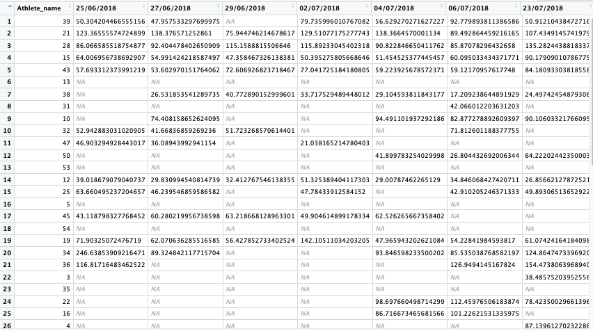
Wide data 
Long Data 
reshape2::melt and tidyr::gather
HRV2 %<>% melt("Athlete_name")meltis useful with basic data frames such as this where we only need to specify the variable used to store values,Athlete_namein this case, and the rest is part of the data we are transforming.
HRV2 %<>% melt("Athlete_name", na.rm=TRUE)
We must remove any NAvalues present which may be due to dates where athletes didn’t record any values. We can do this within ourmeltfunction by including na.rm=TRUE(shown above) or we can do this separately by using HRV2 <- na.omit(HRV2).
When we carry out some wrangling the date type may change away from what we need it to be, in this case it may turn our rMSSD data into a character variable instead of numerical. This be be easily remedied using HRV2$value <- as.numeric(HRV2$value).
Next we will carry out all the majority of our data transforming in a single step, where we will log transform the data, create a rolling average and standard deviation of the log transformed data. Using these values we will add in an upper, lower and a warning threshold based of 1.5sd above or below the rolling average for upper and lower respectively then use 0.75sd below the rolling average for the warning line. This approach is known as Statistical Process Control, Matt Sams has a nice blog on it here and it was also covered in this article.

Script 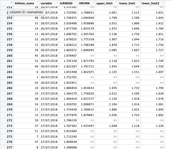
Output
There is a lot happening within the few lines of script so let’s break it down.
- Grouping by athlete with
dplyr::group_by. - Creating a log transformed rMSSD variable called
lnRMSSDthroughdplyr::mutateandlog10. - Standard deviation of the
lnRMSSDvariable calledHRVSDwithsd. "HRVRM"=rollmean(lnRMSSD,7,na.pad=T,align = 'right')creates our 7-day rolling average through thezoo::rollmeanfunction.- Then we multiply our standard deviation by both 1.5 and 0.75 and either add or subtract it from our rolling average to create our upper, lower and warning limit values.
- Finally we remove the original rMSSD and the standard deviation values from our data using
dplyr::select. We do this as we no longer need the data but more importantly it will make plotting the data later an easier task.
Note: We log transform the data as is has been shown to allow better interpretation of rMSSD data (See here and here)
Our next step is to use tidy::gather to take our dataframe spread across a number of columns and reduce to four columns: athlete name; Date; data key; rMSSD value. While we don’t need to take this step, by doing so it allows us to quickly plot the data. If we kept it spread across multiple columns we would have to reference each column separately when it came to plotting the data (although keeping them in separate columns can allow for more customisation when it comes to plotting).


In the above script we use tidyr::gather and look to create a key column which will differentiate between our different values based off our rMSSD data. Then the athlete name and date column (called variable above) will be kept in the same position but their values will be repeated where necessary.
Thats as far as we will go in this blog, next up is going to be putting together our table of the most recent data and then plotting individual plots for each athlete.
Part two of the blog is now available here

One thought on “Analysing and Reporting HRV Data in RMarkdown”