Visuals With R: Multiple Plots

Previously we produced a single plot based off an individual GPS export. In the majority of environments a single plot isn’t of huge value as we could be dealing with over 100 athletes in some environments. The goal of this post will be to outline how we can use facets to produce multiple plots in a quick and efficient manor. This is the plot as we currently know it:

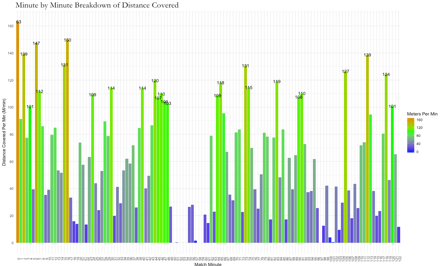
A single plot of a minute by minute breakdown from a game. We have covered analysing multiple raw data GPS exports previously using this script.

In the scenario where we have a low number of athletes to deal with using a basic facet approach where we add facet_grid with the id variable to discriminate between athletes to our plot script will work.

• ggplot(Min_by_min, aes(factor(one_Min), TotalDist_Min, fill=TotalDist_Min))+
geom_bar(stat = 'identity')+
scale_y_continuous(breaks=seq(0,220,20))+
scale_fill_gradient2(low='blue', mid='green', high='red', midpoint = 100, name='Meters Per Min')+
labs(y = "Distance Covered Per Min (M/min)", x = "Match Minute")+
ggtitle("Minute by Minute Breakdown of Distance Covered")+
geom_text(aes(label=ifelse(TotalDist_Min>100, round(TotalDist_Min,0),'')))+
theme_minimal()+
facet_grid(id~.)+
theme(
axis.text.x = element_text(angle=90),
plot.title = element_text(size=20, family = 'Garamond'),
)
• facet_grid(id~.)is saying to create a different plot facets using id to separate between plots, as it comes before the ~  (known as tilde), id will form the different rows of the facet. If it was after the ~, it would plot in columns. The . is saying we don’t want anything forming columns in the facets. We also have the option of having a variable after and before the ~ which would use one to create row and the other to create columns.

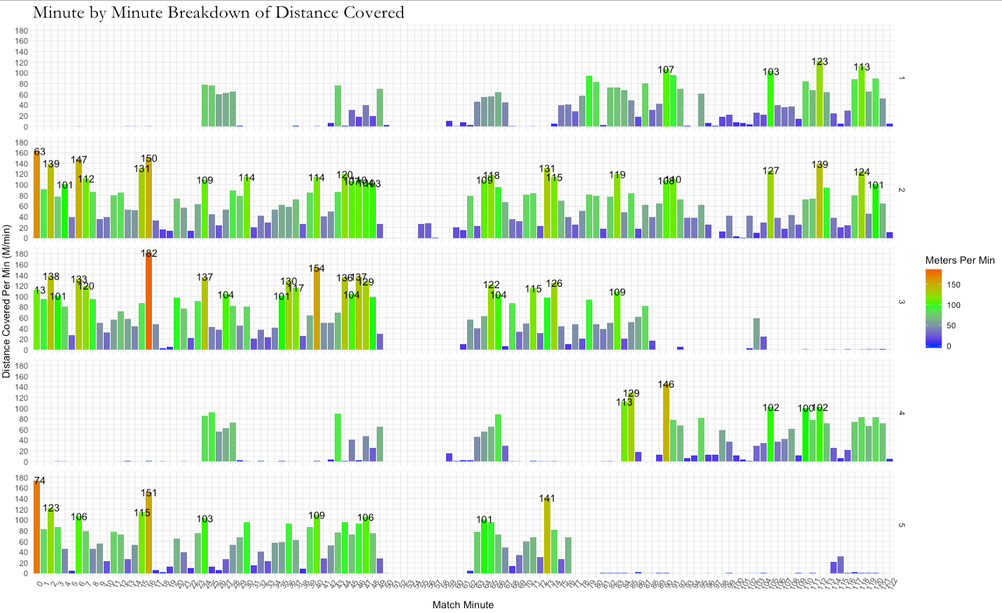
As you can see, producing five separate plots from a raw data export is just as easy as creating a single plot, only a small line separates the two. Working with larger number of athletes can be slightly trickier as using facets can lead to very cramped plots but a similar result can be achieved through a combination of RMarkdown, LaTeX and ggplus, however this will be covered in the next few blogs as it will involve a number of topics.