How To Speed Up Analysis in R: Peak Period Data Extraction

Previously we looked at how to generate a minute by minute profile based off raw GPS data. Today we will go a step further and generate peak period data utilising some of the methods outlined recently on speeding up analysis in r.

First, let’s go through the difference between the two approaches. A minute by minute profile is showing the distance covered in each minute of the session. However, if there was a period of high activity which took place over second 30-60 of minute 10 and second 0-30 of minute 11, it would not be isolated and the data from the this period of high activity would be spread over two minutes. Instead we can generate rolling sums across the whole session from the 10Hz data i.e. sum up the distance covered per 600 data points (10Hz > 10 points per second > 600 points per minute) across the session. The difference in the two approaches can lead to very different peak period readings where the minute by minute data can underestimate peak periods by unto 50m/min. 

Much of our script will be shortened through the use of functions, these functions are going to be stored on a separate script and then brought into our working script through source(). To highlight some of the ways the speed has being improved I will show a number of methods and where feasible the times taken for each with our dataset. 

Loading Files

We are going to look at three difference functions to load in the files here: data.table::fread, reads::read_csv and then base r read.csv. The method to read the files into a single data frame will be by creating a list of the file names and then using purrr::map_dfto create a dataframe of them. We will also include a section that brings the filename itself into the dataframe as a new column so we can differentiate between files. In this case, we can also use tidyr::separate to pull the filename apart then create a column for athlete’s name and session name. 

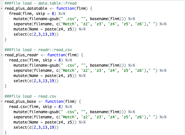
Lets take a deeper look at one of these to explain what the function itself is doing

• fread(flnm, skip = 8)
  • Using fread, read the file (here called flnm within the function) and skip the first 8 lines as they are not needed
• mutate(filename=gsub(” .csv”, “”, basename(flnm)))
  • Create a column called filename using the original name of the file read in
• separate(filename, c(‘Match’, ‘z2’, ‘z3’, ‘z4’, ‘z5’, ‘z6’),” “) 
  • Pull the filename apart into different columns (named above) based on where a space (” “) occurs in the name
• mutate(Name = paste(z4, z5))
  • Pull the two columns involving the names together to create a name column
• select(c(2,3,13,19))
  • Only retain the columns needed for our anlaysis
    • Can lead to improvements in speed when dealing with very large datasets

• 

• 

As can be seen, the data.table::fread has a speed advantage over the two other functions, with the base r read.csv last by a considerable amount. 

Create distance based metrics

This is a similar approach to how it was done previously with a few small changes to account for the fact that the more files analysed, the greater the potential for error to be introduced. We account for this by having limits on how much time can be between each data point. 

• mutate(“SpeedHS” = case_when(Velocity <= 5.5 ~ 0, Velocity > 5.5 ~ Velocity),”SpeedSD” = case_when(Velocity <= 7 ~ 0, Velocity > 7 ~ Velocity))
  • Using mutate and dplyr::case_whento create different threshold based velocites
• group_by(Match, Name) %>% mutate(Time_diff = Seconds-lag(Seconds))
  • Difference in time grouped by both session and name to prevent one file affecting another
• mutate(Time_diff = case_when(is.na(Time_diff) ~ 0,
  Time_diff < 0 ~ 0, Time_diff > 0.1 ~ 0.1, TRUE ~ Time_diff),
  • Using mutate to account for any errors in the time difference metric. Here we account for any NA, negative time difference or a time difference greater then 0.1s
• Dist = Velocity*Time_diff, Dist_HS = SpeedHS*Time_diff,
  Dist_SD = SpeedSD*Time_diff) %>% ungroup() %>%
  select(c(3,4, 8:10))
  • Finally create our distance metrics through velocity multipled by time, then remove unwanted columns 

• 

Rolling Sum Functions

The next part will be spilt into two pieces. First we will briefly cover the use of the Rcpp package and the function it creates within this script and then how along with the  data.table and parallel package will help speed up the most time consuming piece of the script.

 The above  run_sum_v2 function, created in the C++ programming language and along with the Rcpp package, allows us to use it in the R environment. The main benefit of performing the function in this manner is it leads to a considerable speed increase over similar functions. As can be seen below where we compare the run_sum_v2, zoo::rollsum and RcppRoll::roll_sum functions, with the custom function considerably faster than the other two alternatives. 

• 

• 

We use this function within a data.table as this approach is quicker than using base r or a tidyverse approach. Within the DT we also set key columns. By doing so it sorts the columns which in turns aids grouping them further in the by=(Match, Name). We then use paste0to create the column names for the columns we are looking to create(Note the difference between pasted paste0 is simply paste creates a space between the words we are joining and paste0 does not). Finally we create the columns using parallel::mclapply, this functions works very similar to lapply but allows for the use of parallel computing, spreading the work across multiple cores. This will only speed up data analysis for very large datasets, due to time needed to assign the process to the different cores. When used with a dataset of approximately 1.5million rows, lapply was faster. 

• 

• 

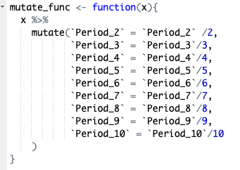
Once we have the rolling sums created for our different variables we need to filter the data so we only retain the highest values for each rolling window. First we remove all the NA values created by the rolling sum using complete.cases(), then remove the columns no longer needed before applying our custom function which all the columns to meters per minute values rather than meters per two minutes, per three minutes etc. Once this is done we group the data by match and name before summarising using dplyr::summarise_at specifying that we want the maximum value for each column. Finally we change the data to long format instead of wide. The final step is beneficial if going on to analyse the data in r, however may be removed if analysing elsewhere.

 Summary File

• 

• 

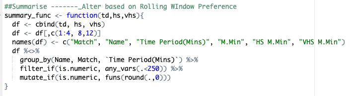
Finally we create a summary file where each of the distance metrics are combined used cbind, then any unnecessary columns removed before filtering for excessively high data (likely to be measurement errors) and rounding the data frame to zero decimal places.

The full script along with a version which includes average acceleration are available on GitHub 

Web-based app, built through R and Shiny, which automates peak period extraction also available here