Exploration of Predictive Analytics: Training Load Prediction

We are going to briefly step away from our recent work around designing a wellness monitoring system (Part I, II & III) and look into a different area, predictive analytics. Recently I posted a link on twitter to a video from a conference last year where a statistician working for a sports analytics company called Orreco outlined their efforts at constructing a training load prediction application. Given the attention it generated I thought I would go through potential steps at replicating the training load prediction.

Laying my cards on the table

First of all, to make my own biases known:

• Statistical analyses of data is not one of my strong points but an area I am working to improve in.
• I have reservations about the use of predictive analytics (PA) within sport science and feel they are often used as main ingredients in a cake rather than the icing on top which may be more reflective of what they offer.
• I feel PA does not often offer more above either basis data manipulation or having sound principals and guidelines in place. Too often the methods are discounted as they are “simple” and don’t have the same “wow” factor as PA.
• Having said the above, I am definitely open to seeing what is possible and having my mind changed about PA in sport.

Basics On Data Used For Analysis

Let’s start with a simple enough analysis and cover basic linear regression where we will look to use total distance covered in a single drill compared to time in seconds. Initially we will spend time carrying out text manipulation, which is new to the blog, to format our data in a more usable manner and hopefully reduce potential for error. As I am using a real dataset here, I won’t always show the results of the analysis however towards the end when it has been reduced and anonymised I will show more.

Info on the dataset used:

• 4 seasons of data split into whole sessions and individual drills
• 855 separate training days
• 158 players present
• Before any cleaning of the data performed it has over 2000 unique named drills/sessions
  • Reduced to 900 after cleaning
• 65 variables in total although we will only use a small number for this demonstration

Initial Data Cleaning

The following steps were carried out before the data was in a format where analysis was possible. This may not be needed for your own data or variations of this may be required:

• Remove data for full sessions so we are left with individual drills only
• Remove any half/quarter match data along with rest periods
• Change drill names to lower-case to prevent conflicts from upper vs lower case
• There is the addition of “3g” at the end of a drill name to note if it was on artificial surface which needs to be removed
  • This could be retained to allow separate analysis for grass vs astroturf
• When the drill has been repeated numerous times across a session it is noted by adding the repetition number at the end, which needs to be removed
• R will differentiate if there is any spaces present at the beginning or end of a phrase, this needs to remove this.
• The drill duration is currently in the “H:M:S” format, to analyse we need to change it to seconds only.

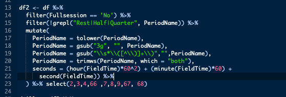
Much of these changes will be carried out using different functions inside either dplyr::filter or dplyr::mutate. Let’s break this down this step:

• filter(Fullsession == 'No')
  • Basic filter here where we keep anything that is not a full session
• filter(!grepl("Rest|Half|Quarter", PeriodName))
  • As we want to remove anything with either half, quarter or rest in it, we use grepl to identify them and then reverse it by using the ! at the beginning
  • Also note the use of |which represents or here
• mutate(PeriodName = tolower(PeriodName)
  • Change all drill names to lowercase
• PeriodName = gsub("3g", "", PeriodName)
  • Remove the “3g” annotation using gsuband replace with nothing
• PeriodName = gsub("\s\([^\)]+\)","",PeriodName)
  • Here we remove the drill number annotation using gsub
• PeriodName = trimws(PeriodName, which = "both")
• Remove trailing or leading whitespace with trimws with which set to both to clear both
• seconds = (hour(FieldTime)60^2) + (minute(FieldTime)*60) + second(FieldTime)))
  • Finally we create our seconds metric by using the hour, minute and second functions from lubridate, converting all to seconds and summing

Further Data Filtering

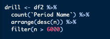
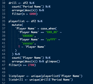
As this is only an exploration into what’s possible, I decided to filter out as much data as possible so I was left with the best chance of arriving at a high level of predictive value. To do this I kept the drill with the highest number of occurrences (n = 6844) along with the player that featured the most in the data (n = 2712). I did this by using dplyr::count along with dplyr::arrange and then filtering all but the highest values. There was a slight difference between the approach used for players and drills, where I first has to correct some misspellings of player names, this was performed through dplyr::case_when. Having created two values, one with the target player and another with the target drill I then filtered my dataset to be left with the desired dataset.

Analysis

Split into Train/Test Data

In order to assess predictive value, we must first separate the data into a training and testing dataset. The model will be built on the training set and then used to predict values which will be compared to our testing dataset. We can carry out this step by using the caTools package in R. This an important step as if you train the model on the same data as you test it on later, it is not a true representation of it’s predictive ability

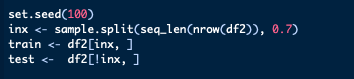
• set.seed(100)
  • This command will allow us to reproduce the analysis as it will ensure the split will always be the same.
• inx <- sample.split(seq_len(nrow(df2)), 0.7)
  • Creates a list of logical values where TRUE will be the case for 70% of the dataset (created by the 0.7).
• train <- df2[inx, ]
  • Create a training dataset equal to 70% of our data
• test <- df2[!inx, ]
  • Create a testing dataset equal to the other 30% of our data

Linear Regression

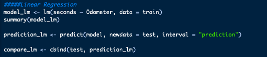
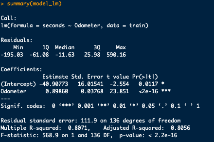
We can create our linear regression using the lm function and compare seconds to our distance variable, odometer. We can view a summary of the regression using the summary function

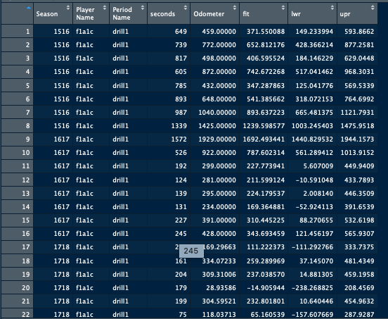
Using the predict function we can create a set of predicted values with the model. Then with cbind add the predicted values to our test dataset in order to compare the two.

Alternatively we can plot the data for a visual comparison

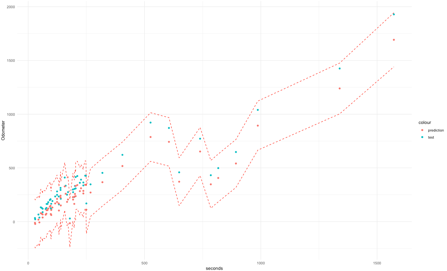
At first glance the data does see to offer a high enough level of predictive values, while the upper and lower limits of the predicted data trend around ±500m, the different between actual and predicted values is usually much lower.

Exploring the results

If we create a variable which represents the difference between the predicted and actual results then plot this variable agains seconds we can see that the model has predicted the distance to ±100m for drill times of up to about 400seconds

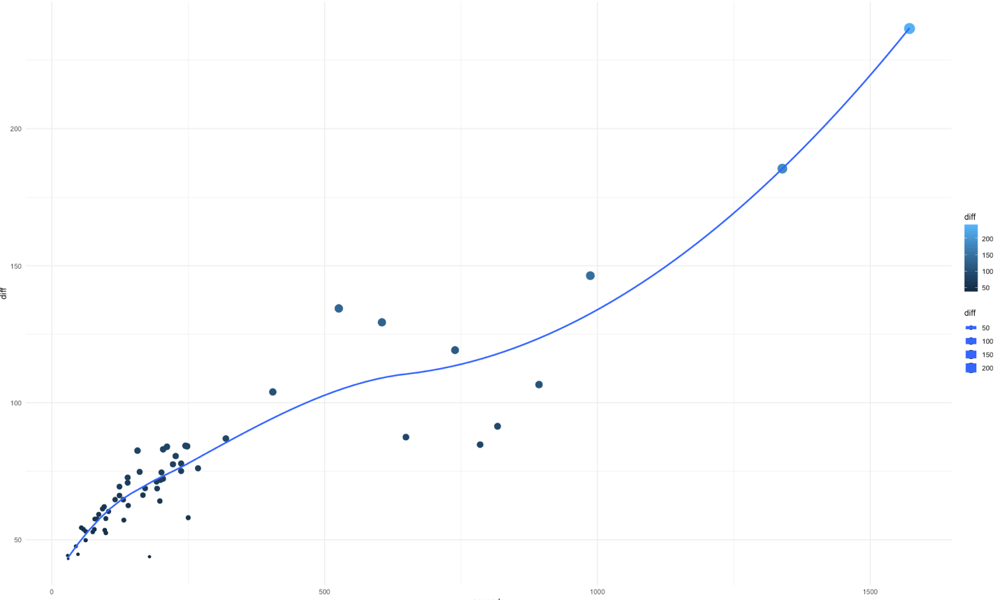
This finding would make sense as the majority of individual repetitions of a drill would be around 2-4 minutes in length with few going past this. In turn this would make the predictive power of the longer drills less accurate. To further illustrate this we can use a simple histogram which further highlights how the majority have a difference of less than 100m.

I replicated this analysis only including drills of less than 400 seconds in length and the difference between the predicted and actual values generally increased. However the AIC was lower for the second analysis so I’m not sure what to infer from this.

Potential Further Steps

• Have a time limit of the data, i.e. only use data from the past 12 months.
  • As this data covers almost 4 years, & the physical profile/demands of a player can change, limiting the data to more recent may improve analysis.
• The majority of the drills are less than 5 minutes in length, having a limit on drill length may increase strength
  • Not the case here however
• Time and distance were chosen to use here, as they are generally highly correlated. Perhaps including more variables and carrying out a different analysis is worth considering.
• Grouping players together to increase volume of data
• Investigate feature scaling and its effects on results

Practical Use?

• Dependant on accuracy desired?
• If this was used for the drill analysed for four repetitions of four minutes, our prediction error would be around ±400m for the whole set
  • Across a 3 day training week this would be around ±1200m
  • A month would be around ±4800m
• At what point is this spread acceptable or not?
• If we performed this analysis for a number of different drills across the day/week/month, how great would our potential error spread be?
• Would it get to the stage that the potential spread was so large to make the analysis nearly void of a practical application?
• What I haven’t mentioned at all, purposely, is the accuracy of the measuring equipment? If the measurement has error in it, this will only be amplified by any work we perform on the data.
• However, the results here definitely show potential!

As an aside, it’s worth noting that the majority of the work above was cleaning the data rather than analysing it. Don’t underestimate the ability to quickly and efficiently clean data!

A version of the script used here is available on GitHub