Principal Component Analysis and Visualisation of Training Load Data

Recently Dan Weaving and the research group at Leeds Beckett University put out a paper outlining how to perform a type of dimension reduction on training load data: principal component analysis (PCA). The benefit of such an analysis is it can reduce a large number of metrics into a more manageable dataset. This may uncover outlier data or trends that were previously difficult/impossible to determine. While the paper itself does a good job of outlining how PCA works and why you may wish to perform it, I wanted to expand upon how to perform PCA here. We will cover the method used within the paper, a package called mdatools that can streamline the analysis and a further method using the tidyverse packages.

However, I would like to point out I do have some reservations about this analysis. While I can see value in the ability to reduce the myriad of metrics we have available to us down to a small number with greater importance. I’m not sure the benefits of the analysis justify the complexity and understanding required to perform the analysis and utilise the output. Even then, can it change or add to your overall process? It may change how you look at the data, does it tell you more than simpler analyses?

While everyone may collect a large number of metrics, decision making usually comes down to a very small number of metrics that can be monitored through more basic methods (note I said monitored not controlled or affected!!). Added to that is the questionable validity of certain metrics already. The SISO principal certainly would apply here. Having said that, I’m more than open to being convinced about its benefit!

Outline of PCA

PCA is particularly useful when working with “wide” data sets i.e lots of variables or metrics. In such datasets, plotting the data in its raw format is not easy which can make it difficult to identify trends or outliers. PCA allows you to see the overall “shape” of the data, identifying which variables/metrics are similar to one another and which are very different. This can enable us to identify groups of datapoints that are similar and work out which variables make one group differ from another. Or in our case, identify which metrics make one training session differ from another.

The mathematics underlying it are somewhat complex and covered within the paper (this blog also covers PCA in an understandable manner), so I won’t go into detail, but the basics of PCA are as follows: you take a dataset with many variables, and you simplify that dataset by turning your original variables into “Principal Components”. Principal Components (PC) are the underlying structure in the data. They indicate where there is the most variance or where the data is most spread out. The first PC shows the most substantial variance in the data and it decreases with each PC from there on.

Eigenvalues/Eigenvectors

Any brief look into PCA will turn up eigenvalues and eigenvectors which may be new to people. Eigenvectors and eigenvalues come in pairs: every eigenvector has a corresponding eigenvalue. An eigenvector is a direction, while an eigenvalue is a number telling you how much variance there is (or how “strong” the variance is) in that direction. Within PCA, the eigenvector with the highest eigenvalue is the first principal component. The number of eigenvalues and eigenvectors within the model is the same as the number of dimensions the data has. We can reframe the data in terms of these eigenvectors and eigenvalues. Reframing a dataset using eigenvalues and eigenvectors does not change the data itself, simply lets us look at it from a different angle, which may represent the data better.

Base Method

(Method outlined by the Weaving et al paper.) Note I am calling this the base method as it involves functions that come with the base version of R and does not require additional packages. This does not imply the analysis itself is of less value. The results are identical throughout, only the script and visual outputs change. Using the datapasta package I have recreated the data from Weaving et al to perform the analysis. The full script along with creating the data is available for download here and will be linked below also. Once created, the data contains 169 days for a single player with a number of metrics and variations of the acute chronic ratio (let’s save THAT discussion for another day).

There are a few ways of performing PCA within base R however here we will use the prcomp() function. Within the prcomp function we use centre = TRUE & scale = TRUE which in essence is z-scoring the data in order to scale/normalise it for analysis. As the first two columns of the Date and Player_ID are not measures of training load we must remove them from our dataset to be analysed, however this can easily be done within the function itself.

• pca.model <- prcomp(df_pca[,-c(1:2)], center = TRUE, scale. = TRUE)

Once the PCA model is created we can access the various components to view their data:

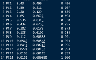
• summary(pca.model)
  • Variance attributable to each principal component
  • General rule of thumb is to include enough principal components to account for roughly 90% of the variance
• pca.model$sdev
  • Normalized singular values
• pca.model.eigvals <- pca.model$sdev^2)
  • Normalized eigenvalues
• pca.model$rotation
  • Eigenvectors
• pca.model$x
  • Principal components

Visuals

We will create plots here using features of base R. As when plotting elements of a PCA model one or more plots tend to be linked and work better when viewed together we will use the par(...) function to create them in the same plot space. Specifically we will use par(mfrow = c(1, 2)) here which creates a plot space for two plots side-by-side in a single row.

As mentioned previously, the variance accounted for by each PC is important. Ideally having 90%+ accounted for by the first 2 or 3 allows them to be quickly analysed using 2D or 3D scatter plots. Lets look at creating some plots to visualise the variance first.

• par(mfrow = c(1, 2))
  • Creates plot space
  • Note this function will continue to operate until either replaced or stopped using dev.off()
• plot(pca.model, type = "l")
  • Variance of Each Component
• plot(cumsum(pca.model.eigvals / sum(pca.model.eigvals)), type="b", ylim=0:1, ylab = "Cumulative variance, %", xlab = "Components")
  • Cumulative Variance
• abline(h=0.9, lty=2)
  • Line indicating 90% cumulative variance

As we can see, the first three principal components account for 90% of the variance. However to simplify the plotting process here, I am going to stick with the first two only (plotly and the gg3d package appear to be the best options for 3D scatterplots in R).

Once we have established which PCs we need to include we move on to exploring our data through them. Here we again create two plots, the first indicates where individual sessions lie in terms of the first two PCs and the second, the loading of each variable on those PCs.

• PC1 <- pca.model$x[,1]
• PC2 <- pca.model$x[,2]
  • Accessing first and second principal component
• rownumb_x <- length(PC1)
• rownumb_y <- length(PC1)
  • Finding row number of last training session to highlight within data
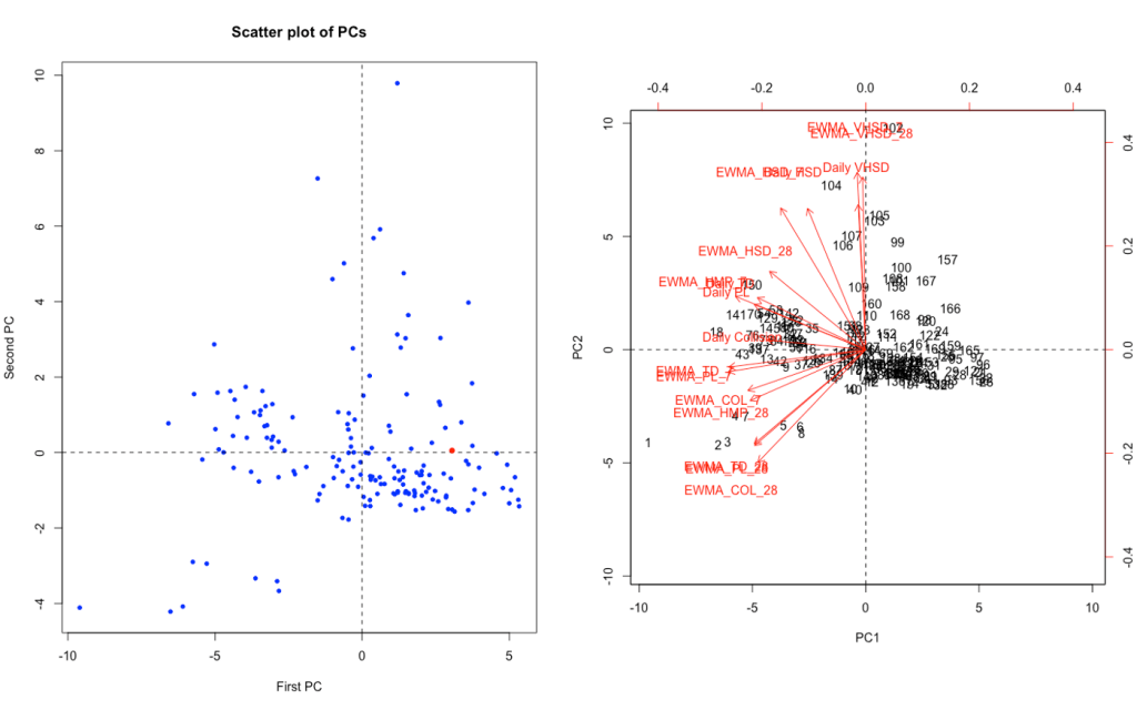
• plot(PC1,PC2, main = "Scatter plot of PCs", pch=20, col="blue", xlab = "First PC", ylab = "Second PC")
  • Scatter plot with recent data highlighted
• abline(h=0, lty=2)
• abline(v=0, lty=2)
  • Adds vertical/horizontal lines where x & y axis are equal to zero
• points(PC1[rownumb_x], PC2[rownumb_y], col="red", pch=16, cex=3)
  • Highlights last recorded session (once data organised chronologically)
  • col= sets point colour, pch= sets point type, cex= sets point size
• biplot(pca.model, scale=0)
  • Biplot with eigenvectors showing
• abline(h=0, lty=2)
• abline(v=0, lty=2)
  • Adds vertical/horizontal lines where x & y axis are equal to zero

We can now see where our most recent session falls and how it relates to our various metrics. The scatterplot on the left indicates the most recent session was about average with no metric/PC in particular standing out. The biplot on the right indicates that for our first two PCs, the greater the y-value/PC2 the more influenced by high-speed running whereas the lower the PC1/x-value the more it seems to relate to collision influenced metrics.

MDAtools Package – PCA

Just as there are a number of methods of performing PCA in base R, there are a number of packages designed to carry out some or all of the analysis. Here we will look at one such package in detail, mdatools by Sergey Kucheryavskiy. This package is an R package for preprocessing, exploring and analysis of multivariate data. While we will use its PCA abilities plus some extra functions, it can also be used for analyses such as Partial Least Squares (PLS) Regression, SIMCA Classification and PLS Discriminant Analysis. This package itself has an online user guide here (it also goes into PCA in much more detail).

Within the script linked, please restart your R session (CMD/CTRL + SHIFT + F10) before running mdatools section as the plotting functions may conflict with earlier work. Following restart, run section to create data. Using mdatools, we can quickly create and visualise our PCA model:

• pca.model2 <- pca(df_pca[,-c(1:2)], center = TRUE, scale = TRUE)
  • Similar to prcomp function
• plot(pca.model2, show.labels = T)
  • Creates autoplot of key PCA visuals

Now we see how our first two PCs affect the data, how our metrics relate to them and the cumulative variance of our PCs. Finally we also have a new plot which shows outliers using two distance metrics created from the results of a PCA model.

The first is distance from original position of an object to the PC space, known as Q-distance. The Q-distance shows how well datapoints fit the model which allows us detect points that do not fit well. The second distance is known as Hotelling T² distance or a score distance. The T² distance allows to us to see how much variance is present within a single training day, (i.e majority of metrics may be average but some may be unusually high/low). The plot also includes limits for outlier detection using these distances. The mdatools guide has a section dedicated to residuals and limits in a PCA model.

While these visuals are good in that they give us a quick overview of our data. We can create them separately using the different plot functions which also lets us customise them to a greater degree.

• par(mfrow = c(1, 2))
  • Creating our plot space (1 row X 2 columns)
• plotVariance(pca.model2, type = "b", variance = "expvar", main = "Variance", xlab = "Components", ylab = "Explained variance, %", show.legend = F)
  • Using the plotvariance() function to show the variance of each PC set by variance = "expvar"
• plotVariance(pca.model2, type = "b", variance = "cumexpvar", main = "Cumulative Variance", xlab = "Components", ylab = "Cumulative variance, %", show.legend = F)
  • Using the plotvariance() function to show the variance of each PC set by variance = "cumexpvar"

• mdaplot(pca.model2$calres$scores, type = 'p', show.labels = T, show.lines = c(0, 0))
• mdaplot(pca.model2$loadings, type = 'p', show.labels = T, show.lines = c(0, 0))
  • These create our first two plots from the four shown above.
  • Outlining how each day and each metric relates to PC1 and PC2

However we can add features to these plots to increase their value and interpretability.

• par(mfrow = c(2, 2))
  • Create 2×2 plot space
• plotScores(pca.model2, c(1, 2), show.labels = T, cgroup = df_pca$Daily HSD, labels = df_pca$Date)
  • Plots each session for the first two PCs
  • Colours them according to the daily high speed distance (can be any metric here)
  • Labels them by date
• plotLoadings(pca.model2, c(1, 2), show.labels = T)
• plotResiduals(pca.model2, cgroup = df_pca$Daily HSD, labels = df_pca$Date, show.labels = T)
  • Colours them according to the daily high speed distance
  • Labels them by date
• plotVariance(pca.model2, type = 'h', show.labels = T, labels = 'values', show.legend = F)

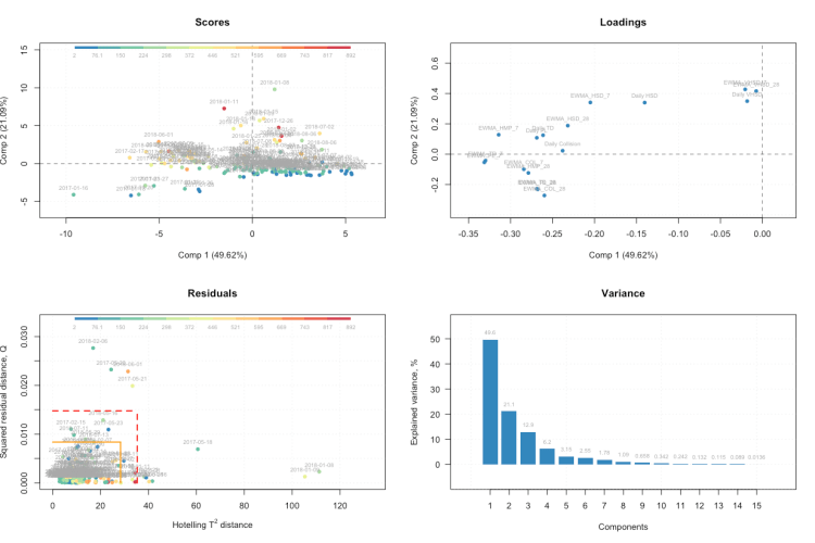
Now within a single plot space we can view how individual sessions and each metric relate to the first two PCs along with identify some potential outliers and relate sessions to high speed distance. Additionally, the fourth plot gives us an indication of the value of the first two PCs in performing the analysis.

Tidyverse Based PCA Method

Having explored both base R and mdatools package, I will present one final option here which utilises the tidyverse group of packages. As many people initially learn R through the tidyverse, having a PCA method with syntax and languages they may be more familiar with can be beneficial. Note this is leaning heavily on the approach outlined by Tyler Bradley here. As we are using the tidyverse packages, we will build our plots using the ggplot2 package. We will also introduce some new functions to the blog that have general uses, particularly the following three:

• tidyr::nest()
  • Creates nested dataframe
• purrr::map() & purrr::map2()
  • Applies function to each element of a data structure
  • In this case, a nested dataframe
  • map2() applies functions to multiple arguments/structures
• broom::augment()
  • Takes output of non-tidyverse based functions and turns them into “tidy” data frames

Creating Our Model

• df_pca2 <- df_pca %>%
  • Access data for analyses
• nest() %>%
  • Created initial nested dataset
• mutate(
• pca = map(data, ~ prcomp(.x %>% select(-c(Date, Player_ID)), center = TRUE, scale = TRUE)),
  • Create our PCA model within a dplyr::mutate using prcomp)
• pca_aug = map2(pca, data, ~augment(.x, data = .y)))
  • Using broom::augment turn our PCA model into a tidy data frame called pca_aug
• This results in a dataframe containing 3 nested data frames:
  • Initial dataset
  • PCA model
  • Tidy PCA model

Variance Analysis

Unlike the previous two approaches, we do need some further data wrangling before we can start to produce our plots in a meaningful manner. Here we will create a separate dataset that will allow us to quickly produce plots of the variance explained by each PC along with the cumulative variance.

• var_exp <- df_pca2 %>% unnest(pca_aug) %>%
  • Access and unnest our tidy PCA model
• summarize_at(.vars = vars(contains("PC")), .funs = funs(var)) %>%
  • Using dplyr::summarise_at() we select the variables containing PC (our principal components) and the corrr::var() function to get the total variance for each PC
• gather(key = pc, value = variance) %>%
  • Arrange them into a long dataset rather than wide
• mutate(var_exp = variance/sum(variance), cum_var_exp = cumsum(var_exp), pc = str_replace(pc, ".fitted",""))
  • Using dplyr::mutate() we get the percentage variance per PC, cumulative variance and then today the names of each PC

Now we have the data to plot the variance and cumulative variance of the PCs in a tidy format as ggplot2 likes to work with!

• var_exp %>% rename(Variance Explained = var_exp,Cumulative Variance Explained = cum_var_exp ) %>%
  • Access data and rename variables so as to be better for plot output
• gather(key = key, value = value, Variance Explained:Cumulative Variance Explained) %>%
  • Change from wide to long format
• mutate(pc = factor(pc, levels = c("PC1", "PC2", "PC3", "PC4", "PC5", "PC6", "PC7", "PC8", "PC9", "PC10", "PC11", "PC12", "PC13", "PC14", "PC15", "PC16", "PC17"))) %>%
  • Create factor variable so PCs occur in correct order
• ggplot(aes(pc, value, group = key)) + geom_point() + geom_line() +
  • Create plot base
• facet_wrap(~key, scales = "free_y") +
  • Facet based on key created earlier
• lims(y = c(0, 1)) +
  • Set y-axis limits (should never go above 1 as we are dealing with percentages here
• geom_hline(yintercept = 0.9) +
  • Horizontal line set at 0.9 y-intercept so as to identify when 90% of variance explained
• labs(title = "Variance explained by each principal component")
  • Set plot title
• bbplot::bbc_style() + theme(axis.text.x = ggplot2::element_text(size=10))
  • Additional theme elements using the bbplot package along with custom text size

Principal Component 1 & 2 Analysis

Next we can look to plot our first two PCs. While the basic plot here is straightforward to produce, as outlined in Tylers blog, to make it slightly more attractive and add meaning to our specific set of data I have a number of additional steps. These include theme alterations, coding data points according to the data and highlighting more recent training days. We will use the ggfortify package as its autoplot() function automates plotting of the output of prcomp within the ggplot2 framework. The plot will be built using a combination of dplyr::mutate() and purrr::map2(), we will have to access the plot at the end using the dplyr::pull() function.

• mean_hsr <- mean(df_pca2[[3]][[1]][[5]])
  • Identify the average high speed running to use for our colour coding later
  • Note as we are accessing data within a nested dataframe it involves the use of square brackets
• df_pca2 %>% mutate(
  • Access data and begin mutate function
• pca_graph = map2(.x = pca, .y = data,
  • Begin map2 function, specifying our PCA model and original data as elements to work over.
• ~ autoplot(.x, loadings = TRUE, loadings.label = TRUE, loadings.label.repel = TRUE, label.label = NULL, data = .y) +
  • Use autoplot to build our plot base. Produces scatterplot of data with eigenvectors (directional arrows) of metrics showing
• geom_vline(xintercept = 0, colour='blue', linetype='dashed') + geom_hline(yintercept = 0, colour='red', linetype='dashed') +
  • Add dashed lines when X and Y axes are equal to zero to give biplot effect
• geom_point(aes(fill=df_pca2[[3]][[1]][[5]]), shape=21) + scale_fill_gradient2(low='blue', mid='green', high='red', midpoint = midpo) +
  • As not all geom_point() shapes will take a fill argument we need to first change the shape to one that will
  • Then apply a colour scale using scale_fill_gradient2()
  • We could also use the size= argument within geom_point() and apply a second metric to it as shown below where Playerload determines size
• labs(title = "First two principal components of PCA on Training Load dataset", subtitle = "Colour Indicates Daily HSR, Recent Days Highlighted") +
  • Set title & subtitle
• ggrepel::geom_label_repel(aes(label=ifelse(df_pca2[[3]][[1]][[2]] >= max(df_pca2[[3]][[1]][[2]]) - days(10), as.character(df_pca2[[3]][[1]][[2]]), ""), fill=df_pca2[[3]][[1]][[5]]), nudge_y = 0.3, size = 4) +
  • Here we create labels using an ifelse() statement where they will only appear if the data is in the last 10 days of recorded data.
  • I did have issues creating the labels as ggrepel() struggled to recognise the data format hence the use of as.character() to over come this.
• bbplot::bbc_style() + theme(legend.key.width = unit(2, "cm"), legend.key.height = unit(1, "cm")))) %>%
  • Set theme features and close mutate
• pull(pca_graph)
  • pull() then ends the pipe by producing the plot

If you are considering adding PCA to your day-to-day work stream, checking out some interactive visuals will definitely help you explore the results of your model!

Now we have covered three methods of performing PCA in R. The pysch package, ggbiplot and FactoMineR packages all have elements dedicated to performing and/or plotting PCA models if you wish to explore further. Finally the caret package is one developed for the tiydverse group of packages to allow a wide range of data modelling.

The full script for all methods shown above is available for download here. The script is completely self-contained and will create data then perform all steps above.

Additional Considerations For PCA

Before finishing I want to quickly cover some additional considerations surrounding PCA:

• Normalising your data is important, even more so if you have variables with very different units such as an AC ratio which hovers around 0.5 – 2.5AU and a total distance metric which can be 10,000m + (i.e. 10^1 vs 10^4)
• How you normalise your data can affect your results (See here)
• PCA is a type of feature extraction – it creates the same number of variables as original dataset but with differing levels of important. On the other hand, factor analysis will reduce the number of features within your dataset.
• Groupings within your data following PCA can be investigated through the geom_ellipse() function
• There are alternative methods available to use here (Kernal PCA & t-SNE are two of the more common), however they may not have the same level of interpretability at the end as PCA and the more advanced the method, the more it is designed for very wide datasets.
• As explained by Weaving et al, tests of sampling adequacy designed for factor analysis can be used to assess the suitability of your data for PCA. See image for Bartletts test and Kaiser-Meyer-Olkin.

library(tidyverse)
library(magrittr)
library(ggfortify)
library(lubridate)
library(broom)
### Creating Data ####
data1 <- c("1/16/2017 13 5255 149 530 0 25", "1/18/2017 13 4367 74 411 0 10", "1/20/2017 13 3569 147 402 0 60", "1/23/2017 13 7234 253 717 0 20", "1/25/2017 13 4420 126 421 0 9", "1/26/2017 13 2929 106 274 0 3", "1/27/2017 13 5135 213 549 0 39", "1/28/2017 13 1784 49 157 0 2", "1/30/2017 13 3019 643 331 19 8", "2/5/2017 13 4790 199 479 1 17", "2/7/2017 13 3382 242 340 74 8", "2/8/2017 13 2316 69 193 0 4", "2/9/2017 13 6149 392 602 0 67", "2/11/2017 13 2764 144 307 12 6", "2/13/2017 13 6002 254 686 91 26", "2/15/2017 13 2584 189 229 2 6", "2/16/2017 13 2033 148 169 0 0", "2/17/2017 13 7506 541 814 8 73", "2/23/2017 13 1927 110 170 0 1", "2/24/2017 13 5162 310 550 10 56", "3/28/2017 13 3014 83 245 0 0", "3/30/2017 13 1642 43 147 0 0","4/6/2017 13 2498 2 251 0 0", "4/11/2017 13 3545 580 288 0 0", "4/13/2017 13 2957 144 238 0 0", "4/14/2017 13 5467 248 555 0 41", "4/17/2017 13 5033 293 465 16 25", "4/24/2017 13 2467 103 203 0 0", "4/26/2017 13 2392 119 201 0 2", "4/27/2017 13 5283 376 555 1 48", "5/4/2017 13 2993 209 291 5 9", "5/6/2017 13 8022 486 836 20 89", "5/11/2017 13 3361 192 352 0 16", "5/13/2017 13 1897 120 188 0 2", "5/14/2017 13 6983 438 639 38 44", "5/17/2017 13 4294 452 395 20 3", "5/18/2017 13 2885 163 560 0 89", "5/20/2017 13 1485 166 127 0 1", "5/21/2017 13 8118 362 705 13 66", "5/23/2017 13 2103 14 252 0 4", "5/25/2017 13 3068 153 288 0 1", "5/26/2017 13 5817 313 643 13 55", "5/29/2017 13 7682 446 808 9 74", "6/6/2017 13 3846 307 336 0 1", "6/8/2017 13 3092 188 285 0 5","6/9/2017 13 2233 161 194 1 0", "6/10/2017 13 5859 612 589 25 58", "6/13/2017 13 3588 201 347 0 1", "6/15/2017 13 2578 121 231 0 0", "6/16/2017 13 6130 370 608 15 47","6/22/2017 13 1687 86 151 0 0", "6/23/2017 13 7113 473 742 56 60","6/28/2017 13 1856 41 152 0 0", "6/29/2017 13 8201 702 825 26 68","7/4/2017 13 3327 135 324 0 6", "7/6/2017 13 3642 206 373 0 11","7/8/2017 13 2179 153 201 0 0", "7/9/2017 13 7848 552 738 53 49", "7/11/2017 13 3012 179 291 0 8", "7/13/2017 13 2120 189 196 0 0","7/14/2017 13 1135 88 110 0 10", "7/19/2017 13 3193 83 318 0 2","7/21/2017 13 2942 105 310 0 0", "7/24/2017 13 3913 230 410 6 0","7/26/2017 13 3208 251 304 2 12", "7/28/2017 13 1910 148 173 2 3", "7/29/2017 13 3811 299 386 33 34", "8/1/2017 13 4292 583 384 0 7","8/3/2017 13 2726 199 242 1 0", "8/4/2017 13 7602 497 742 31 73","8/7/2017 13 3058 128 334 0 4", "8/9/2017 13 2683 160 215 0 0","8/10/2017 13 6456 479 675 3 69", "8/15/2017 13 1811 93 176 0 3","8/17/2017 13 2840 176 245 4 0", "8/18/2017 13 7823 546 849 6 80","8/27/2017 13 3029 208 324 1 15", "8/28/2017 13 2852 163 280 0 9", "8/30/2017 13 2143 185 199 10 1", "8/31/2017 13 7086 472 705 29 61","9/4/2017 13 4008 185 394 0 28", "9/5/2017 13 2290 130 224 0 16","9/7/2017 13 2219 137 204 9 2", "9/8/2017 13 6243 476 666 12 64", "9/12/2017 13 3394 217 318 10 4", "9/14/2017 13 2087 131 167 0 0","9/15/2017 13 4590 203 473 0 45", "9/21/2017 13 1398 107 100 0 0", "9/25/2017 13 3441 114 324 0 0", "9/26/2017 13 2597 135 227 5 2", "9/28/2017 13 1941 140 168 0 2", "9/29/2017 13 7130 466 726 9 63","10/6/2017 13 1677 119 135 0 0", "10/7/2017 13 7889 404 795 20 71","11/19/2017 13 4223 194 449 0 0", "12/18/2017 13 2465 151 204 0 0", "12/19/2017 13 1213 237 105 0 0", "12/23/2017 13 3334 629 276 0 3", "12/26/2017 13 2719 891 239 97 0", "1/2/2018 13 3377 861 310 39 0", "1/5/2018 13 3084 640 272 20 0", "1/8/2018 13 3802 234 364 399 1",
"1/9/2018 13 3501 364 306 0 0", "1/11/2018 13 4418 848 388 55 0", "1/15/2018 13 3260 482 294 112 0", "1/16/2018 13 4425 388 395 0 0", "1/18/2018 13 2841 553 255 41 0", "1/23/2018 13 2188 511 222 28 14",
"1/25/2018 13 4099 456 387 0 8", "1/28/2018 13 4868 153 439 18 7", "1/30/2018 13 3330 103 301 0 0", "2/1/2018 13 4455 228 457 1 21", "2/4/2018 13 2225 50 218 0 3", "2/6/2018 13 4670 208 418 0 6",
"2/7/2018 13 1812 76 165 0 0", "2/8/2018 13 5033 316 563 0 55", "2/12/2018 13 4453 166 424 0 2", "2/14/2018 13 4160 205 394 17 13", "2/16/2018 13 3020 209 340 18 37", "3/26/2018 13 4890 644 458 0 0",           "3/29/2018 13 1270 16 130 2 3", "3/31/2018 13 3125 448 287 0 0", "4/2/2018 13 6043 290 602 22 36", "4/5/2018 13 3186 92 275 0 0", "4/6/2018 13 2573 140 232 0 0", "4/8/2018 13 7805 511 793 21 58", 
"4/10/2018 13 2789 142 226 0 1", "4/12/2018 13 2437 222 208 6 0", "4/13/2018 13 7131 450 766 35 56", "4/18/2018 13 2293 202 208 8 0", "4/25/2018 13 4863 206 434 0 5", "4/26/2018 13 1007 9 131 0 9",
"4/27/2018 13 3555 229 312 0 5", "4/29/2018 13 5653 227 616 16 66", "5/2/2018 13 3733 256 368 0 7", "5/3/2018 13 1703 70 167 0 0", "5/4/2018 13 6958 447 771 0 77", "5/7/2018 13 4604 372 502 0 30", 
"5/8/2018 13 3189 184 295 0 0", "5/10/2018 13 3123 306 281 20 5", "5/11/2018 13 7375 521 755 42 50", "5/15/2018 13 6206 632 635 25 8", "5/16/2018 13 4392 291 395 0 6", "5/18/2018 13 2150 146 191 0 0", 
"5/19/2018 13 6822 423 701 8 0", "5/23/2018 13 4238 290 431 6 4", "5/26/2018 13 7635 469 823 1 0", "5/29/2018 13 3504 251 347 27 3", "5/31/2018 13 1825 66 327 2 42", "6/1/2018 13 7349 569 725 103 48",
"6/4/2018 13 3196 159 347 63 0", "6/8/2018 13 2369 148 261 62 27", "6/12/2018 13 2006 117 184 0 0", "6/14/2018 13 2783 191 277 1 0", "6/20/2018 13 1546 286 177 0 0", "6/29/2018 13 1640 8 191 0 0",
"7/2/2018 13 1696 486 177 163 0", "7/4/2018 13 5212 350 504 35 0", "7/7/2018 13 1816 35 175 0 0", "7/8/2018 13 5040 483 535 10 0", "7/11/2018 13 2541 160 236 1 0", "7/12/2018 13 2904 121 287 0 7", "7/13/2018 13 6001 286 665 0 80", "7/16/2018 13 2540 133 268 0 1", "8/2/2018 13 1757 381 148 0 0", "8/6/2018 13 2201 244 228 96 9", "8/6/2018 13 2201 244 228 96 9", "8/7/2018 13 3159 146 328 0 13", "8/11/2018 13 3317 93 368 0 0")
data2 <- c( "5255 5255 149 149 530 530 0", "4048 4856 102 134 402 488 0", "3169 4456 94 126 327 451 0", "3146 4095 103 119 317 413 0", "2874 3854 89 112 284 387 0", "2888 3790 94 112 281 379 0","3450 3883 123 119 348 391 0", "3033 3738 105 114 300 375 0", "2461 3449 220 143 252 348 5", "1636 2577 89 107 165 260 1", 
"1765 2467 110 109 178 248 19", "1903 2456 100 107 181 245 14", "2965 2711 173 126 287 269 11", "2359 2541 133 119 238 255 9", "2827 2616 138 121 305 268 28", "2236 2446 125 118 229 248 16", "2185 2417 131 120 214 243 12", "3516 2768 234 149 364 282 11", "1107 1936 69 105 107 195 2", "2121 2158 129 119 218 220 4", 
"754 427 21 18 61 39 0", "834 484 22 18 71 44 0", "736 466 4 11 72 44 0", "1061 570 146 48 89 51 0", "1336 698 118 51 110 60 0", "2369 1027 150 65 221 94 0", "2258 1176 137 73 209 108 4", "918 883 44 51 79 80 1", "1114 931 55 53 95 83 0", "2157 1231 135 75 210 115 1", "1036 953 70 60 101 90 1", "2588 1379 161 85 266 136 6", "1454 1197 86 73 151 119 1", "1292 1168 78 71 132 116 1", "2715 1569 168 97 259 152 10", 
"2219 1562 184 109 208 150 9", "2386 1654 179 113 296 178 7","1713 1536 142 109 198 163 4", "3314 1990 197 127 325 201 6","2390 1870 114 111 246 191 4", "2111 1832 103 107 210 186 2", "3038 2107 155 121 318 217 5", "3202 2230 177 128 336 231 4", "1282 1524 94 94 118 154 0", "1494 1535 100 94 137 153 0", "1679 1583 115 99 152 156 0", "2724 1878 239 134 261 186 7","2046 1763 151 122 197 174 3", "1796 1706 115 114 168 166 2", 
"2879 2011 179 132 278 197 5", "934 1426 53 92 87 139 1", "2479 1818 158 118 251 180 15", "1052 1400 48 85 98 137 3", "2839 1869 211 128 279 184 9", "1506 1537 84 99 147 151 2", "1758 1584 99 100 176 157 1", "1533 1523 94 97 149 150 1", "3112 1959 208 128 296 190 14", "2504 1906 162 124 240 185 8","1938 1798 138 120 184 174 4", "1737 1753 126 118 165 169 3","1211 1446 51 88 119 140 1", "1416 1457 55 84 144 143 0",
"1576 1445 81 83 163 144 2", "1688 1474 108 90 168 146 2", "1427 1410 98 88 138 138 1", "2023 1575 148 103 200 155 9","1927 1567 208 123 180 152 4", "1765 1546 167 120 162 148 3", "3224 1964 249 146 307 189 10", "2125 1796 137 127 213 176 4", "1866 1742 117 121 174 167 2", "3014 2067 208 146 299 202 3", "1168 1571 72 108 115 154 1", "1367 1558 85 106 126 150 1", "2981 1990 200 136 307 198 3", "981 1255 67 86 104 127 0", 
"1449 1365 91 91 148 137 0", "1351 1331 97 92 133 133 3", "2784 1728 191 118 276 172 9", "1883 1575 107 102 186 156 3","1985 1624 113 104 195 161 2", "1671 1561 98 99 161 154 4", "2814 1884 192 125 287 189 6", "1739 1649 115 109 170 164 4", "1500 1574 97 103 138 154 2", "2272 1782 124 110 221 176 2", "754 1257 49 79 64 121 0", "1099 1182 44 67 101 114 0", "1473 1279 67 72 133 121 1", "1314 1243 73 72 117 117 1", 
"2768 1649 171 99 269 159 3", "789 1115 53 68 70 106 0","2564 1583 140 92 251 153 5", "1056 365 48 18 112 38 0", "617 216 38 13 51 19 0", "766 285 88 28 65 25 0","1076 444 185 64 89 38 0", "1134 546 301 113 97 47 24","996 564 256 128 93 51 13", "1191 668 268 148 107 60 11","1453 801 171 135 136 74 104", "1965 987 220 151 179 90 78", "2210 1161 335 189 197 104 58", "1514 1097 227 176 136 99 46","2242 1326 267 190 201 119 35", "1971 1346 288 203 177 121 30", "1015 1092 196 177 97 100 14", "1596 1230 224 185 152 113 8",
"1890 1328 133 160 174 122 8", "1896 1381 101 146 173 126 4", "2180 1504 113 142 212 141 3", "1476 1367 60 118 144 129 1", "1998 1507 86 117 216 151 1", "1951 1528 83 114 203 152 0", "2722 1770 141 128 293 180 0", "1974 1637 86 107 199 165 0", "2151 1706 100 107 210 170 4", "1965 1687 108 107 203 171 7","1222 449 161 52 115 43 0", "833 450 72 43 81 44 0", "1250 605 152 68 117 58 0", "2214 942 158 79 216 91 6", "1730 980 90 70 160 93 2", "1941 1089 102 75 178 102 2","3043 1483 185 100 298 143 6", "2409 1478 140 97 224 140 3",            "1964 1449 134 99 178 136 3", "3256 1841 213 123 325 179 11","1346 1446 101 100 129 140 5", "1395 1212 65 75 126 115 1","1298 1198 51 70 127 116 0", "1862 1361 95 81 173 129 0","2461 1569 110 86 251 155 4", "1971 1524 111 87 198 150 2","1904 1536 101 86 190 151 1", "3168 1910 187 111 335 194 1","2487 1859 172 115 267 191 0", "2663 1951 175 120 274 198 0","2279 1906 175 125 224 191 5", "3553 2284 261 152 357 230 14",            "2676 2144 241 158 272 217 11", "3105 2299 253 167 303 229 8","2284 2141 179 155 218 212 5", "3419 2464 240 173 339 245 5", "2141 2144 148 150 215 214 3", "2812 2256 180 154 296 230 2", "2062 2063 139 141 212 209 7", "1616 1914 95 127 201 204 5", "3050 2289 213 158 332 240 29", "2086 2068 130 138 227 217 28",
"1252 1717 78 114 137 181 24", "898 1428 54 94 89 149 8", "1201 1430 78 94 120 148 4", "600 1038 85 81 66 109 1", "455 659 8 43 66 76 0", "616 649 125 68 72 74 41", "1649 922 158 83 167 98 32", "1150 869 75 70 114 92 13","2122 1157 177 98 219 122 13", "1531 1109 115 90 151 115 5","1874 1233 116 92 185 127 4", "2906 1561 159 106 305 164 3","1861 1435 100 95 196 151 1", "453 547 96 54 38 55 0", "694 563 91 58 69 57 24", "1071 676 130 71 109 69 42", "1593 847 134 76 164 87 31", "1333 865 66 63 144 91 10")
data3 <- c( "0 1008 1008 25 25", "0 753 925 17 22", "0 685 874 24 24","0 675 812 15 20", "0 535 746 11 18", "0 508 724 9 17", "0 607 737 16 19", "0 507 700 13 18", "1 543 678 9 16", "1 316 502 6 11", "6 323 475 5 10", "5 329 467 5 10", "5 567 523 20 14", "5 500 503 13 13", "11 611 527 14 13","9 487 496 9 11", "9 458 488 7 11", "9 765 570 23 15", "6 215 393 4 10","6 436 442 17 13", "1 98 72 0 1", "1 97 74 0 1", "0 55 56 0 1", "0 231 100 0 0", "0 242 117 0 0", "0 414 173 10 3", "1 382 197 11 4", "1 125 140 1 3", "1 191 155 1 2", "1 446 228 13 6", "1 230 185 4 4", "2 559 279 24 10", "1 300 241 10 8", "1 265 236 6 7", "4 542 314 16 9",
"4 486 325 7 8", "4 528 347 28 13", "4 381 324 16 12", "4 610 391 28 15", "4 398 354 17 14", "3 351 342 10 12", "4 572 404 21 15", "4 654 440 27 17","2 283 308 3 10", "2 298 305 3 9", "2 318 311 2 8", "3 586 385 16 12", "3 400 353 7 9", "2 337 337 4 8", "3 546 394 15 11", "2 159 274 3 7", "6 515 364 17 11", "4 181 271 4 8", "6 623 387 20 12", "4 319 318 6 9", "3 367 327 6 8", "3 296 308 4 7", "6 613 395 15 10", "6 527 393 10 9","5 391 366 6 8", "4 361 360 7 8", "3 193 281 2 6", "3 344 309 1 5","3 374 312 1 4", "2 377 317 3 4", "2 296 298 3 4", "4 472 346 10 6", "4 500 362 6 5", "3 423 353 3 5", "5 728 442 21 9", "4 483 405 10 8", 
"4 370 378 6 7", "4 651 455 21 11", "2 242 343 6 8", "2 274 335 3 7","3 681 443 22 12", "1 231 283 5 7", "1 315 302 6 7", "2 285 292 4 7", "4 620 384 18 10", "3 382 339 13 10", "3 402 348 14 10", "3 351 336 8 9", 
"4 634 415 22 13", "3 361 356 8 10", "3 282 330 4 8", "3 434 369 15 11", "2 136 257 3 7", "1 248 249 1 5", "2 308 266 1 5", "1 274 258 1 5","2 603 350 17 9", "1 160 234 2 5", "2 511 326 19 10", "0 213 74 0 0", 
"0 216 69 0 0", "0 245 87 0 0", "0 460 171 1 0", "7 552 237 0 0", "7 447 247 0 0", "7 427 265 0 0", "33 456 290 0 0", "31 582 336 0 0", "30 730 402 0 0", "31 462 366 0 0", "29 690 435 0 0", "28 638 446 0 0", 
"21 376 374 4 1", "18 575 425 4 1", "16 517 418 3 2", "14 455 408 2 1","12 515 425 6 3", "10 342 378 3 2", "9 461 401 4 3", "8 449 402 3 3","7 628 455 16 6", "6 416 401 6 5", "6 444 406 6 5", "6 422 399 13 7",
"0 270 101 0 0", "0 179 99 1 1", "0 357 157 0 0", "2 512 222 9 3","2 375 223 4 2", "1 419 246 3 2", "3 668 332 16 6", "2 533 331 9 5","2 464 332 5 4", "5 782 429 18 8", "4 316 336 4 6", "2 272 267 2 4", 
"2 240 259 4 4", "2 370 293 4 4", "3 538 345 19 8", "2 440 337 10 7", "2 422 340 7 7", "2 726 429 25 11", "2 570 419 18 11", "1 577 431 13 11", "3 488 419 9 9", "5 812 513 19 12", "6 650 494 8 10", "5 746 531 8 10", "5 537 493 4 8", "5 778 563 3 8", "4 502 493 2 6", "3 690 530 1 5", "5 484 481 1 4", "4 341 436 11 6", "11 684 524 20 9", "13 471 473 9 8", "14 287 394 9 8", "11 197 325 3 6", "9 282 329 2 5", "6 217 260 0 3", 
"3 82 155 0 2", "14 223 177 0 1", "14 377 223 0 1", "12 188 188 0 1","11 479 268 0 1", "9 339 254 0 1", "9 376 270 2 1", "8 618 344 21 7", "7 381 311 9 5", "2 130 127 0 2", "8 254 154 2 2", "14 404 203 4 2", "13 504 244 6 3", "10 159 183 2 2")
df1 <- tibble::enframe(data1, name=NULL)
df2 <- tibble::enframe(data2, name=NULL)
df3 <- tibble::enframe(data3, name=NULL)
df1 %<>% separate(value, into =c("Date", "Player_ID", "Daily TD", "Daily HSD", 
                          "Daily PL", "Daily VHSD", "Daily Collision"), sep=" ")
df2 %<>% separate(value, into =c("EWMA_TD_7", "EWMA_TD_28", "EWMA_HSD_7", 
                          "EWMA_HSD_28", "EWMA_PL_7", "EWMA_PL_28", 
                          "EWMA_VHSD_7"), sep=" ")
df3 %<>% separate(value, into =c("EWMA_VHSD_28", "EWMA_HMP_7", "EWMA_HMP_28",  
                          "EWMA_COL_7", "EWMA_COL_28"), sep=" ")
df_all <- bind_cols(df1, df2, df3)
df_all %<>% mutate(Date = as.POSIXct(as.character(Date), format="%m/%d/%Y",tz=Sys.timezone(), origin="1970-01-01")) %>% mutate_at(c(2:19), as.numeric)
########## PCA Stuff #####
df_pca <- df_all 
### Standard Method
pca.model <- prcomp(df_pca[,-c(1:2)], center = TRUE, scale. = TRUE)
summary(pca.model)                      # This displays the variance attributable to each principal component.
pca.model$sdev                          # This displays the normalized singular values.
(pca.model.eigvals <- pca.model$sdev^2) # These are the normalized eigenvalues.
pca.model$rotation                      # These are the eigenvectors.
pca.model$x                             # These are the principal components.
# Produce a scatter plot of the scores for the first two principal components.
par(mfrow = c(1, 2))
plot(pca.model, type = "l") ###Variance of Each Component
plot(cumsum(pca.model.eigvals / sum(pca.model.eigvals)), type="b", ylim=0:1, 
     ylab = "Cumulative variance, %", xlab = "Components") ### Cumulative Variance
abline(h=0.9, lty=2) ### Line indicating 90% cumulative variance
PC1 <- pca.model$x[,1]
PC2 <- pca.model$x[,2]
rownumb_x <- length(PC1)
rownumb_y <- length(PC1)
### Scatter plot with recent data highlighted
plot(PC1,PC2, main = "Scatter plot of PCs", pch=20, col="blue", xlab = "First PC", ylab = "Second PC")
abline(h=0, lty=2)
abline(v=0, lty=2)
points(PC1[rownumb_x], PC2[rownumb_y], col="red", pch=16, cex=3)
## Biplot with eigenvectors showing
biplot(pca.model, scale=0)
abline(h=0, lty=2)
abline(v=0, lty=2)
points(PC1[rownumb_x], PC2[rownumb_y], col="red", pch=16)
dev.off()
###mdatools package ####
# Restart R before continuing (ctrl/cmd + shift + f10) then run the code to create data but skip base r methods
library(mdatools)
pca.model2 <- pca(df_pca[,-c(1:2)], center = TRUE, scale = TRUE)
plot(pca.model2, show.labels = T)
par(mfrow = c(1, 2))
plotVariance(pca.model2, type = "b", variance = "expvar", main = "Variance", xlab = "Components", ylab = "Explained variance, %", show.legend = F)
plotVariance(pca.model2, type = "b", variance = "cumexpvar", main = "Cumulative Variance", xlab = "Components", ylab = "Cumulative variance, %", show.legend = F)
par(mfrow = c(1, 2))
mdaplot(pca.model2$calres$scores, type = 'p', show.labels = T, show.lines = c(0, 0))
mdaplot(pca.model2$loadings, type = 'p', show.labels = T, show.lines = c(0, 0))
par(mfrow = c(2, 2))
plotScores(pca.model2, c(1, 2), show.labels = T, cgroup = df_pca$`Daily HSD`, labels = df_pca$Date, )
plotLoadings(pca.model2, c(1, 2), show.labels = T)
p2 <- plotResiduals(pca.model2, cgroup = df_pca$`Daily HSD`, labels = df_pca$Date, 
              show.labels = T, lim.col = c("orange", "red"),
              lim.lwd = c(2, 2), lim.lty = c(1, 2))
plotVariance(pca.model2, type = 'h', show.labels = T, labels = 'values', show.legend = F)
### Tidyverse Method ####
df_pca2 <- df_pca %>% 
  nest() %>% 
  mutate(pca = map(data, ~ prcomp(.x %>% select(-c(Date, Player_ID)), center = TRUE, scale = TRUE)),
         pca_aug = map2(pca, data, ~augment(.x, data = .y)))
var_exp <- df_pca2 %>% 
  unnest(pca_aug) %>% 
  summarize_at(.vars = vars(contains("PC")), .funs = funs(var)) %>% 
  gather(key = pc, value = variance) %>% 
  mutate(var_exp = variance/sum(variance),
         cum_var_exp = cumsum(var_exp),
         pc = str_replace(pc, ".fitted", "")) 
## Plot variance
var_exp %>% rename(`Variance Explained` = var_exp, `Cumulative Variance Explained` = cum_var_exp) %>% 
  gather(key = key, value = value, `Variance Explained`:`Cumulative Variance Explained`) %>% 
  mutate(pc = factor(pc, 
                levels = c("PC1", "PC2", "PC3", "PC4", "PC5", "PC6", "PC7",
                           "PC8", "PC9", "PC10", "PC11", "PC12", "PC13", "PC14",
                           "PC15", "PC16", "PC17"))) %>%
  ggplot(aes(pc, value, group = key)) + 
  geom_point() + 
  geom_line() + 
  facet_wrap(~key, scales = "free_y") +
  lims(y = c(0, 1)) +
  geom_hline(yintercept = 0.9) +
  labs(title = "Variance explained by each principal component") +
  bbplot::bbc_style() +
  theme(axis.text.x = ggplot2::element_text(size=10))
mean_hsr <- mean(df_pca2[[3]][[1]][[5]])
df_pca2 %>%
  mutate(pca_graph = map2(.x = pca,.y = data,
      ~ autoplot(.x, loadings = TRUE, 
                 loadings.label = TRUE, loadings.label.repel = TRUE, label.label = NULL, data = .y) +
        geom_vline(xintercept = 0, colour='blue', linetype='dashed') +
        geom_hline(yintercept = 0, colour='red', linetype='dashed') +
        geom_point(aes(fill=df_pca2[[3]][[1]][[5]], size=df_pca2[[3]][[1]][[6]]), shape=21) +
        scale_fill_gradient2(low='blue', mid='green', high='red', midpoint = mean_hsr) +
        labs(title = "First two principal components of PCA on Training Load dataset",
             subtitle = "Colour = Daily HSR, Size = PlayerLoad, Recent Days Highlighted") +
        ggrepel::geom_label_repel(aes(
          label=ifelse(df_pca2[[3]][[1]][[2]] >= 
                         max(df_pca2[[3]][[1]][[2]]) - days(10),
                       as.character(df_pca2[[3]][[1]][[2]]), ""), 
          fill=df_pca2[[3]][[1]][[5]]),
          nudge_y = 0.3, size = 4) +
        bbplot::bbc_style() +
        theme(legend.key.width = unit(2, "cm"), legend.key.height = unit(1, "cm")))) %>%
  pull(pca_graph)
library(psych)
library(REdaS)
r <- cor(df_pca[,-c(1:2)])
nObs <- nrow(df_pca[,-c(1:2)])
cortest.bartlett(r, n=nObs)
KMOS(df_pca[,-c(1:2)], use = "pairwise.complete.obs")