How to Overcome Messy Excel Sheets in R

**Largely Inspired by many a painful Excel sheet along with Duncan Garmonsways (@nacnudus) Spreadsheet Munging Strategies & recent linked presentation

It’s not unusual as a practitioner to be in the position where you get landed an Excel sheet or a number of them often organised in unusually formatted tables with little recognisable structure. This may be due to you taking over a pre-existing project or perhaps helping an external organisation with some work. While a single sheet formatted like that can be managed easily with some copy and paste, as the number of sheets build this becomes a very inefficient and frustrating approach. Thankfully, some kind souls have helped vastly improve this process with a number of helpful packages available.

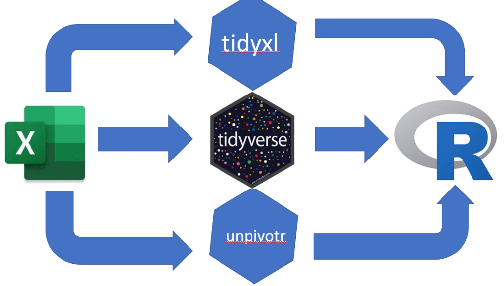
We have two packages that will do the majority of the work for us:

• unpivotr
  • Deals with messy tables, formatting, multi-headed tables etc.
• tidyxl
  • Useful package in general for .xlsx based data
  • Particularly the xlsx_cells() function which reads the excel sheet in cell by cell. The resulting dataframe has a row per sheet cell with a number of variables about the cells

Plus, thankfully, both can be implemented with the tidyverse group of packages.

Messy Excel Sheet Samples

There are a couple of ways in which an excel sheet can be difficult to deal with:

• Multiple Headers/Tables
• Summary Values
• Merged cells
• Empty cells in needless places

Strategies for Dealing With a Messy Excel Sheet

Depending on the format of the excel sheet or sheets you are looking to work on here, how you can tidy it and create a set of data to use in R or elsewhere will differ. However there are a number of general steps that can be taken.

‘for’ loops

‘for’ loops allow you to repeat a sequence of instructions when certain conditions are met. This may be for unique values in a vector or variable, items present within a list or in our situation, read a number of Excel files together or a number of sheets present within an Excel spreadsheet. To do so there are a small number of steps which we will initially cover separately and then at the end show how they can combined through nested for loops.

*There may be a method of using the purrr package in place of for loops however it’s not a package I’m very familiar with (yet).

First to read a number of Excel files in, which within R looks like the following:

list_file <-list.files('Excel Files', pattern='(^[A])(?:.+)(*.xlsx)')
a <- list()
for(p in 1:length(list_file)){
file_path <- paste0('Excel Files/',list_file[[p]])
cells <- xlsx_cells(file_path)
a[[file_path]] <- cells
}

• Here we have looked in a file called Excel Files
• Identified files beginning with a capital A and ending in .xlsx
  • pattern='(^[A])(?:.+)(*.xlsx)'
  • The ^ symbol implies starting with, * implies ending with.
  • (?:.+) means both conditions must be met.
• Use a for loop to read them into the list called a.
  • Using the tidyxl::xlsx_cells() function which reads in every cell in the sheet as a separate line in a dataframe.
  • We used paste0 to create the file path as we currently only have the file name.
  • We then name the newly created dataframe in the list after the file path.

tidyxl::xlsx_cells()

The xlsx_cells() function has a column which identifies which excel sheet the data has come from. Using this variable and the split() function we can then create another list which will contain a dataframe for each sheet within the list.

excel_list <- split(cells, cells$sheet)

Now we are in a position where we we can have all our excel files read in quickly and then separate then into separate data frames. This puts us in a position where if our files are all formatted in the same way we can iterate through them easily with a single for loop.

Next we will look at the steps and functions available to us in order to go from having data frames that aren’t easy to analyse to nicely formatted tidy dataframes. First, however, lets have a look at how our data frames are structured. With the function we used to read in the sheets we end up with the following variables:

• sheet
  • Which sheet within the excel file is the cell present
  • As above can be used to separate out different sheets or remove certain sheets with filter()
• address
  • The location of the cell within the sheet i.e. A1, B6 etc.
• row
  • What row the sheet is in
  • Can remove or select certain rows using this
• col
  • What column the sheet is in
  • Can remove or select certain column using this
• is_blank
  • Is there data of any form present within the cell
  • Depending on your sheet, you may want to remove any empty cells straight away
• data_type
  • What type of data is present from the following: blank, character, numeric, date or error value
  • Lets you filter out or keep certain data types only
• error
  • What is the error value (e.g. #DIV/0! for a dividing by zero error )
• logical
  • Is there a logical value present (Usually output of if/and/or functions)
• numeric
  • What the numeric value of the cell is
• date
  • The data time value of the cell
• character
  • The character string present within the cell
• Along with a number of others:
  • character_formatted, formula, is_array, formula_ref, formula_group, comment, height, width, style_format, local_format_id

For our work we will only need to focus on the first few variables: sheet, character, numeric, date, row, col, data_type. With these we can reformat our data into the desired format. Much of the others may be more useful if looking to see how an excel sheet has been constructed rather than working within R.

Selecting certain sheets, rows or columns

Selecting particular sheets, rows or columns in r tend to follow a similar approach. From the dataframe containing our sheet information use the filter function to either remove or retain the desired data. This is a useful step to reduce the work needed to identify specific tables within a sheet where multiple may exist. As much as possible, removing unneeded cells makes it easier to today your data. An example of this may look like the following example:

rows_remove <- c(18, 19, 48, 49, 78, 79, 108, 109 )
cells %<>%
select(sheet, character, numeric, date, row, col, data_type) %>%
filter(sheet != 'Sheet 1' & sheet != 'Sheet 2' & sheet != 'Sheet 3') %>%
filter(!row %in% rows_remove & row < 122) %>%
filter(col < 30)

• Here we have created a vector of row values we wish to remove.
• Selected the variables we want to keep using select(),
• Removed sheets we do not want with filter()
  • With this filter call we use != which means not equal to
• Use %in% to remove row values equal to our earlier created values and ones less than 122.
  • We also use ! at the beginning of the filter call which reverses the filter to remove certain rows whereas without it, the function would keep those rows.
• Remove any columns which are numbered greater than 30.

Identifying table headers with unpivotr::behead()

Here we will use the behead() function and direct it where to look for the header using North/South/East/West directions. Admittedly, I’m not 100% sure on the use of this function and usually opt for the trial and error approach of working through the directions until I find the header I want in the right place! I have found it best to remove any unwanted data from the dataframe using the above methods before looking to arrange the data in the desired fashion first. This makes it easier to identify table headers as there is less overall clutter in the data.

table_2 <- tl_table %>%
behead("N", 'header_row') %>%
behead('W', 'row_name') %>%
filter(header_row != 'LOAD') %>%
select(sheet, row_name, header_row, numeric) %>%
arrange(header_row)

Here we have created both a table header column and a row name column using the behead() function before finally selecting the desired columns with select() and arranging based on data within the header_row column with arrange().

Within the behead() function we identify the direction that the desired header row lies in the data. As we have separated the data into its different tables and remove much of the clutter before this step, we simply need to indicate where the header row lies. For us, as the header row lies at the top, we use “N” to indicate the north direction. Similarly as the row names are to the left within the data, we use “W” to indicate this. The full range of directional calls allowed are: "N", "E", "S", "W", "NNW", "NNE", "ENE", "ESE", "SSE", "SSW". "WSW" and "WNW" which may be needed for more disordered tables. Following the direction call we indicate the name we would like to assign our newly created variable within our data.

Final Arranging of Data

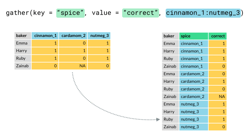
Finally we rearrange our data into the desired end format using one or both of tidyr::pivot_wider() or tidyr::pivot_longer() (for those unfamiliar, these are recently updated versions spread() and gather()). These functions let us arrange our data from long (many rows) to wide (many columns) or vice-versa. Here we will use pivot_wider() to rearrange our newly created header_row variable so that it lies along the top of our data as a header row should.

df1_tl <- bind_rows(a) %>%
filter(complete.cases(.)) %>%
pivot_wider(names_from = 'header_row', values_from = 'numeric')

We have a few steps occurring here so lets walk through them:

• Combining data within a list to a single dataframe
  • If as mentioned earlier you created a list to store data frames in, bind_rows() can be used to turn the list of data frames into a single dataframe once they all have the same formats.
  • rbind() can be used here also however bind_rows() is more efficient
• Removing NA values
  • Here we use a combination of filter() and complete.cases() to remove any missing values
• Rearranging from long to wide
  • Using this function we need only identify which column contains our variable names, names_from and which contains the data we wish to rearrange, values_from.

One function which I haven’t mentioned here but may of value to people is tidyxl::xlex(). When applied to a cell containing a function in Excel, this function gives an indication of how nested that Excel function may be. Heavily nested Excel functions are often the source of pain for many and having the ability to explore them easily is invaluable! There is a more in-depth exploration of this function available to read here.

In Closing

Hopefully I have provided the basics for you to attack and behead 😉 your messy spreadsheets here. Soon I will provide a sample messy spreadsheet and talk through how it can be rearranged using the above methods. Don’t forget, if you would like to learn more about this, Duncan Garmonsway has an awesome resource available to read here.